On this page
- What is the core economic trade-off of skipping hardbanding?
- Which input variables do you need before running the downtime math?
- How do you calculate the real cost of hardbanding per joint?
- What does one extra wear-related trip actually cost?
- Why does casing wear dominate the model as a tail risk?
- How do bare and hardbanded tool joints compare side by side?
- Which variables actually drive the hardbanding decision?
- How should you structure the hardbanding cost worksheet?
- Key Takeaways
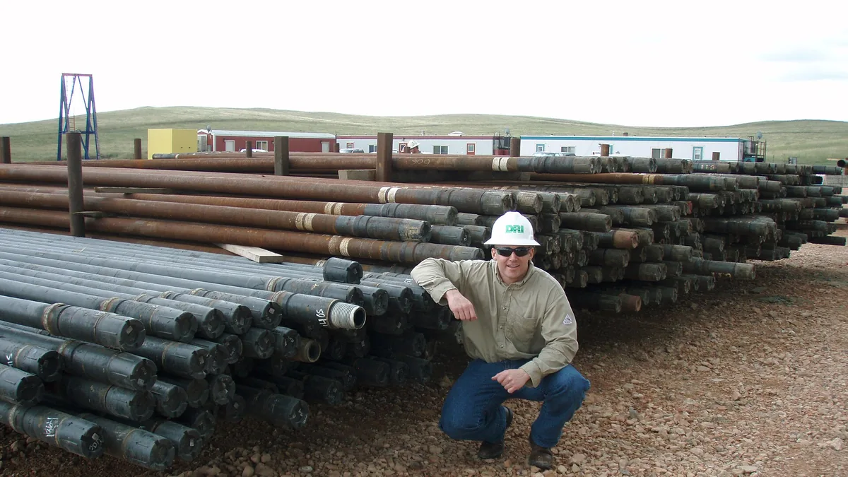

Skipping hardbanding looks like a saving only until you add the cost of the trips it forces, the casing it wears, and the rig days it burns. A single unplanned trip on a modern spread often costs more than hardbanding an entire drill string, and one casing wear failure can exceed the annual hardbanding budget of a mid-size fleet. This article gives you a transparent, parametric worksheet so you can run the numbers with your own day rates instead of trusting a vendor’s comparison.
Every formula below uses variables, not fixed prices, because day rates, alloy costs, and trip times vary wildly between land rigs in West Texas and platform operations offshore. If you can fill in a spreadsheet, you can build this model in an afternoon.
What is the core economic trade-off of skipping hardbanding?#
The core economic trade-off of skipping hardbanding is a comparison between a certain, front-loaded spend and a probability-weighted uncertain loss. Hardbanding cost per joint is known and amortizable, while the cost of skipping includes the probability-weighted sum of extra trips, casing repair, tool joint replacement, and rejected pipe. If the cost of skipping exceeds the cost of protection even at conservative probabilities, hardbanding pays for itself.
Hardbanding is a known, front-loaded cost. The losses it prevents are probabilistic: not every unprotected string will trip early, and not every worn tool joint will score casing. That asymmetry is why the decision gets deferred, and why it shouldn’t be.
The economics reduce to one comparison:
- Cost of protection (C_p): hardbanding spend per joint, amortized over the number of wells or rotating hours the deposit survives.
- Cost of skipping (C_s): the probability-weighted sum of extra trips, casing repair, tool joint replacement, and rejected pipe.
If C_s exceeds C_p even at conservative probabilities, hardbanding pays for itself. The sections below build each term so you can plug in real numbers. For background on why tool joints wear in the first place, see Why Drill Pipe Tool Joints Wear Out.
Which input variables do you need before running the downtime math?#
Before running any downtime math, you need to collect a defined set of input variables from your own operation: rig spread rate, trip time, joint count, hardbanding cost per joint, alloy cost, deposit weight, shop labor rate, arc-on time, tool joint replacement cost, casing wear repair cost, wear-event probabilities, and deposit life in wells. Do not use industry averages for the final decision, only for sanity checks while you build the model.
| Variable | Definition | Typical Source |
|---|---|---|
| R_d | Rig spread rate, $/day | AFE or daily cost report |
| R_h | Spread rate, $/hour (R_d / 24) | Derived |
| T_trip | Round-trip hours to pull and rerun a string | Tour sheets, historical tripping data |
| N_j | Number of joints in the string | String records |
| C_hb | Hardbanding cost per joint | Shop quote, or built up below |
| C_alloy | Alloy consumable cost, $/lb | Supplier invoice |
| W_dep | Deposit weight per joint, lb | Deposit geometry and density |
| L_shop | Shop labor and machine rate, $/hr | Shop cost accounting |
| T_arc | Arc-on plus handling time per joint, hr | Timed trials or shop data |
| C_tj | Cost to replace or refurbish one tool joint | OEM quote or shop rate |
| C_cw | Casing wear repair cost per event | Workover or squeeze quote |
| P_trip | Probability of at least one wear-related trip per well | Your failure and inspection history |
| P_cw | Probability of a casing wear event per well | Your own records or offset data |
| N_wells | Wells drilled between hardband applications | Deposit life tracking |
A note on probabilities: if you have no internal history, start pessimistic. Assume P_trip of 0.3 per well in abrasive formations and P_cw of 0.1 in deviated holes with casing across the wear zone. Then sensitivity-test the model by doubling and halving each probability. If the decision flips when you halve a probability, you have found the variable worth measuring properly.
How do you calculate the real cost of hardbanding per joint?#
The real cost of hardbanding per joint is built from alloy consumables, shop labor and arc-on time, preparation, and quality assurance, not from the shop’s flat per-joint quote. Handling, preparation, and arc-on time usually dominate consumables, so machine deposition and efficient shop flow matter more than shaving cents off alloy price. The string total is the per-joint cost multiplied by the joint count, amortized over the deposit’s useful life in wells.
C_hb = (C_alloy × W_dep) + (L_shop × T_arc) + C_prep + C_qa
Where C_prep covers blasting, cleaning, OD measurement, and preheat fuel, and C_qa covers inspection and documentation. For procedure details that drive these costs, see Hardbanding Welding Procedure: Preheat to Cool-Down.
Rules of thumb for the buildup:
- Consumables are rarely the dominant term. Handling, preparation, and arc-on time usually are, which is why machine deposition and efficient shop flow matter more than shaving cents off alloy price.
- A full hardband band on a 5-inch tool joint typically deposits a modest fraction of a pound per pass; multi-pass bands multiply both alloy and time.
- Quote everything per joint, then multiply by N_j for the string total.
String hardbanding cost: C_string = C_hb × N_j
Amortize it over the deposit’s useful life:
C_amortized = C_string / N_wells
If a deposit survives three wells before needing reapplication, the effective per-well protection cost is a third of the string cost. Re-application over existing deposits changes this math, and is covered in Re-Applying Hardband Over Existing Deposits.
What does one extra wear-related trip actually cost?#
One extra wear-related trip costs the hourly spread rate multiplied by the round-trip hours to pull and rerun the string, and the spread rate keeps running the entire time the string is out of the hole. In a parametric example at $120,000 per day ($5,000 per hour) and a 14-hour trip, one wear-related trip costs $70,000 before any repair cost. Worn tool joints rarely fail one at a time, so the trip often becomes a full string inspection event.
Cost of one wear-related trip: C_trip = R_h × T_trip


Work a parametric example. Say your spread rate is R_d = $120,000/day, so R_h = $5,000/hour. Pulling a 10,000 ft string, inspecting the worst joints, and rerunning takes T_trip = 14 hours:
C_trip = $5,000 × 14 = $70,000
That is one trip, before any repair cost. And worn tool joints rarely announce themselves one at a time; if the wear band at the top of the string is gone, the whole string is suspect, so the trip becomes a full inspection event.
Which ancillary trip costs do most models forget?#
Most models forget four ancillary trip costs: inspection time to gauge every tool joint OD while racked, flat-spot repair or joint replacement plus freight, re-run delay from missing replacement joints, and hole-condition risk that can compound into a stuck pipe or fishing event. Each ancillary cost is added at the hourly spread rate or per-event cost, and hole-condition risk can be modeled as a separate probability term.
- Inspection time: gauge the OD of every tool joint while the string is racked. Add those hours at R_h.
- Flat-spot repair or joint replacement: N_rejected × C_tj, plus freight both ways.
- Re-run delay: if replacement joints are not on site, add standby hours or freight expediting.
- Hole-condition risk: an extra trip in an unstable hole can compound into stuck pipe, which converts a $70,000 trip into a $500,000+ fishing event. Model this as a separate probability term if your hole conditions warrant it.
Expected trip cost per well: E_trip = P_trip × (C_trip + N_rejected × C_tj + ancillaries)
If P_trip is 0.3 and the trip package is $90,000, the expected cost is $27,000 per well, every well, forever, until the root cause is fixed.
Why does casing wear dominate the model as a tail risk?#
Casing wear dominates the downtime model because a bare steel tool joint rubbing against casing in a dogleg or deviated section removes casing wall faster than any designed wear margin, turning an operating nuisance into a capital event. A worn tool joint with a rough, gouged OD is worse than a smooth one because it cuts rather than polishes. Even a low probability of casing wear multiplied by a catastrophic repair cost justifies protection.
The cost stack for a casing wear event:
- Detection and diagnosis: logging to confirm wall loss, often during a trip you did not plan.
- Repair: squeeze cement, patch, or in the worst case, re-drilling and re-casing the section. Even the cheap end of this range dwarfs a hardbanding budget.
- Lost production or delayed TD: the well delivers late, and the rig keeps burning day rate through the repair.
Expected casing wear cost per well: E_cw = P_cw × C_cw
The honest difficulty is that C_cw has a long tail. A minor squeeze might cost a few hundred thousand dollars; a collapsed or pierced intermediate string in a deep well can cost multiples of that plus the well itself. This is precisely the situation where expected-value thinking matters most: even a low P_cw multiplied by a catastrophic C_cw justifies protection.
Alloy selection also matters here. Abrasive hardbands protect the tool joint but can attack casing; casing-friendly alloys sacrifice some deposit life to protect the casing. That trade-off has its own decision framework in Casing-Friendly vs Abrasive Hardband Alloys, and the underlying wear mechanisms are explained in How Hardband Alloys Resist Abrasion Downhole.
How do bare and hardbanded tool joints compare side by side?#
Bare and hardbanded tool joints compare through a single subtraction of expected costs per well: hardbanded joints carry an upfront and amortized protection cost, while bare joints carry the full expected extra trip cost, expected casing wear cost, higher tool joint replacement frequency, and more inspection downgrades. A quality hardband shifts the overwhelming majority of tool joint wear from the joint OD to the deposit, so a conservative protection factor of 0.8 to 0.9 is a reasonable input to sensitivity-test.
Once you have the terms, the comparison is a single subtraction. Build it as a table and let the numbers argue.
| Cost Element | Bare Tool Joints | Hardbanded Tool Joints | How to Compute |
|---|---|---|---|
| Upfront spend | $0 | C_string | C_hb × N_j |
| Amortized protection cost per well | $0 | C_amortized | C_string / N_wells |
| Expected extra trip cost per well | E_trip | E_trip × (1 - protection factor) | P_trip × trip package |
| Expected casing wear cost per well | E_cw | E_cw × (1 - protection factor) | P_cw × C_cw |
| Tool joint replacement | Higher frequency | Lower frequency | N_rejected × C_tj per event |
| Inspection rejects at program end | More joints downgraded | Fewer downgrades | Inspection records |
The “protection factor” is the honest unknown. A quality hardband does not reduce wear risk to zero, but it shifts the overwhelming majority of tool joint wear from the tool joint OD to the deposit. Use 0.8 to 0.9 as a conservative range, then sensitivity-test.
Net benefit per well = (E_trip + E_cw + replacement savings) × protection factor - C_amortized
If that number is positive at your conservative inputs, the decision is made. If it is marginal, the next section tells you where to spend your effort.
Which variables actually drive the hardbanding decision?#
Three variables drive the hardbanding decision in most sensitivity runs: the rig spread rate, the casing wear terms (probability and consequence), and deposit life in wells. High spread rates justify hardbanding almost automatically, deviated wells with intermediate casing across the build section make casing wear dominate, and a deposit that survives five wells amortizes five times better than one that survives one. Alloy selection and application quality, not price, are the biggest levers on the protection side.
Run the model three times: best case, expected case, and worst case. Then vary one input at a time and watch the net benefit. In practice, three variables dominate:
- R_d, the spread rate. Offshore and high-spec land rigs make every avoided hour worth so much that hardbanding is nearly always justified. Cheap workover rigs weaken the case for full-string hardbanding but strengthen it for the bottom-hole assemblies that see the most wear.
- P_cw and C_cw, the casing wear terms. In vertical wells with no casing across abrasive zones, casing wear risk is low and the trip-cost terms carry the argument. In deviated wells with intermediate casing across the build section, casing wear dominates everything else in the model.
- N_wells, deposit life. A deposit that survives five wells amortizes five times better than one that survives one. This makes alloy selection and application quality, not price, the biggest lever on the protection side. Poor application that cracks or spalls the deposit shortens N_wells and silently doubles your effective cost, which is why inspection discipline matters; see Hardbanding Inspection and Acceptance Criteria.
What is the break-even spread rate for full-string hardbanding?#
The break-even spread rate is the point where one avoided wear-related trip pays for the entire string’s hardbanding, calculated as the string hardbanding cost divided by the product of the protection factor and trip time, multiplied by 24. If your actual spread rate exceeds the break-even, one avoided trip pays for the whole string. On most modern spreads, it does, comfortably.
A practical decision rule that falls out of most sensitivity runs: hardband at least the lower third of the string and all BHA connections on any well with abrasive formation or deviation above roughly 10 degrees, and consider full-string hardbanding whenever R_d exceeds the point where one avoided trip pays for the whole string. Solve for that point:
Break-even spread rate: R_d(break-even) = (C_string / (protection factor × T_trip)) × 24
If your actual R_d exceeds the break-even, one avoided trip pays for the entire string’s hardbanding. On most modern spreads, it does, comfortably.
How should you structure the hardbanding cost worksheet?#
Structure the hardbanding cost worksheet in five ordered blocks in a spreadsheet, with one column per scenario (bare, partial hardband, full hardband): an inputs block with all defined variables, a protection cost block, a loss cost block, a net block showing expected total cost per well, and a sensitivity block that multiplies the wear probabilities by 0.5 and 2.0. Keep the model versioned and update it with real inspection data after every well.
- Inputs block: all variables from the definitions table.
- Protection cost block: C_hb buildup, C_string, C_amortized.
- Loss cost block: E_trip, E_cw, replacement frequency.
- Net block: expected total cost per well for each scenario.
- Sensitivity block: multiply P_trip and P_cw by 0.5 and 2.0; recompute.
Keep the model versioned and update it with real inspection data after every well. The single biggest improvement most operators can make is replacing assumed probabilities with their own measured wear rates, which turn the model from a persuasive argument into a management tool.
Key Takeaways#
- One avoided trip pays for full-string hardbanding on most modern spreads; solve the break-even spread rate formula with your own numbers to confirm.
- Build hardbanding cost per joint from alloy weight, arc-on time, and shop labor, not from a flat quote; handling and preparation usually dominate consumables.
- Expected loss is probability times consequence: low-probability casing wear with catastrophic consequence still justifies protection.
- The three variables that drive the answer are spread rate, casing wear exposure, and deposit life, which makes alloy selection and application quality worth more than price shopping.
- Update the model with your own inspection data after every well; measured wear rates beat assumed probabilities every time.
- Drill pipe hardbanding
- Drill pipe tool joint
- Casing wear
- Tool joint hardbanding alloy
- Bottom-hole assembly